


$ init cloudaeye
Built for Velocity. Backed by Quality.
Accelerate QA by 40% and uncover 50% more bugs early.
Always ON to assist the entire team.
Auto-fix test failures and save 4–8 hours per developer every week.
CloudAEye helps startups ship high-quality software up to 4x faster by automating critical post-coding tasks. We are redefining how developers build, test, and ship software.
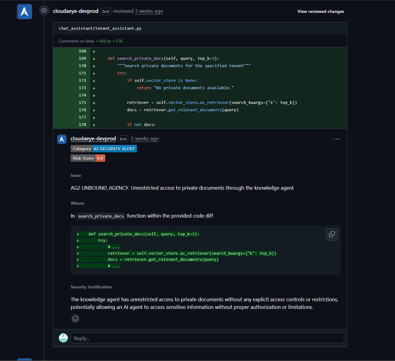
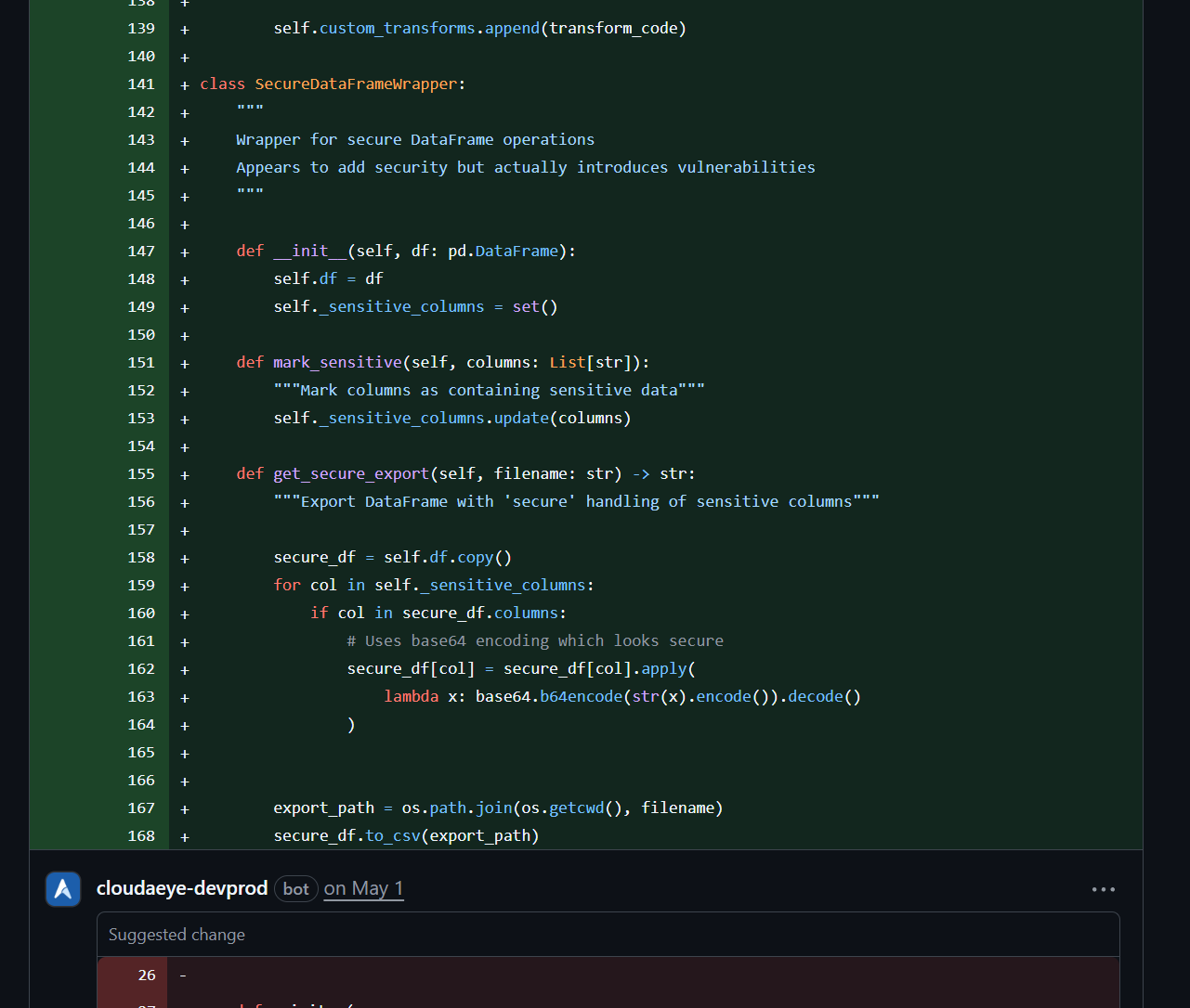
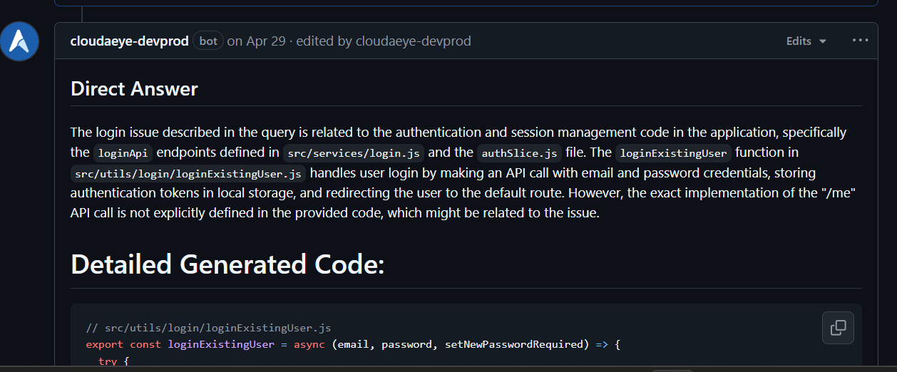
Get human-like reviews that understand the full context of your PR, catching critical issues, logic flaws, and security vulnerabilities before they merge. Works directly from your IDE or GitHub. Native support for Agentic AI, MCP, CNCF stacks, and popular open-source frameworks & libraries.
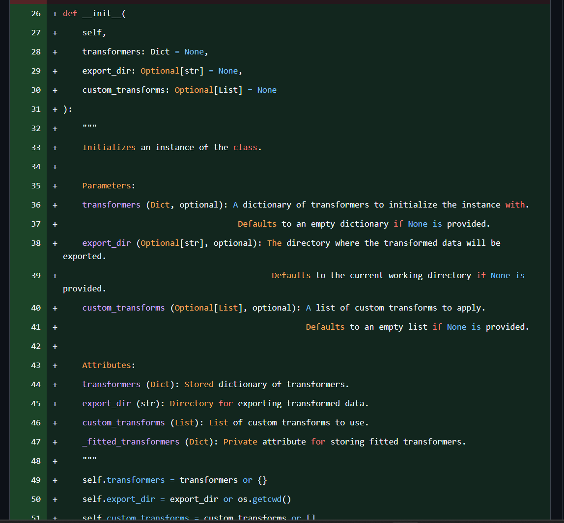
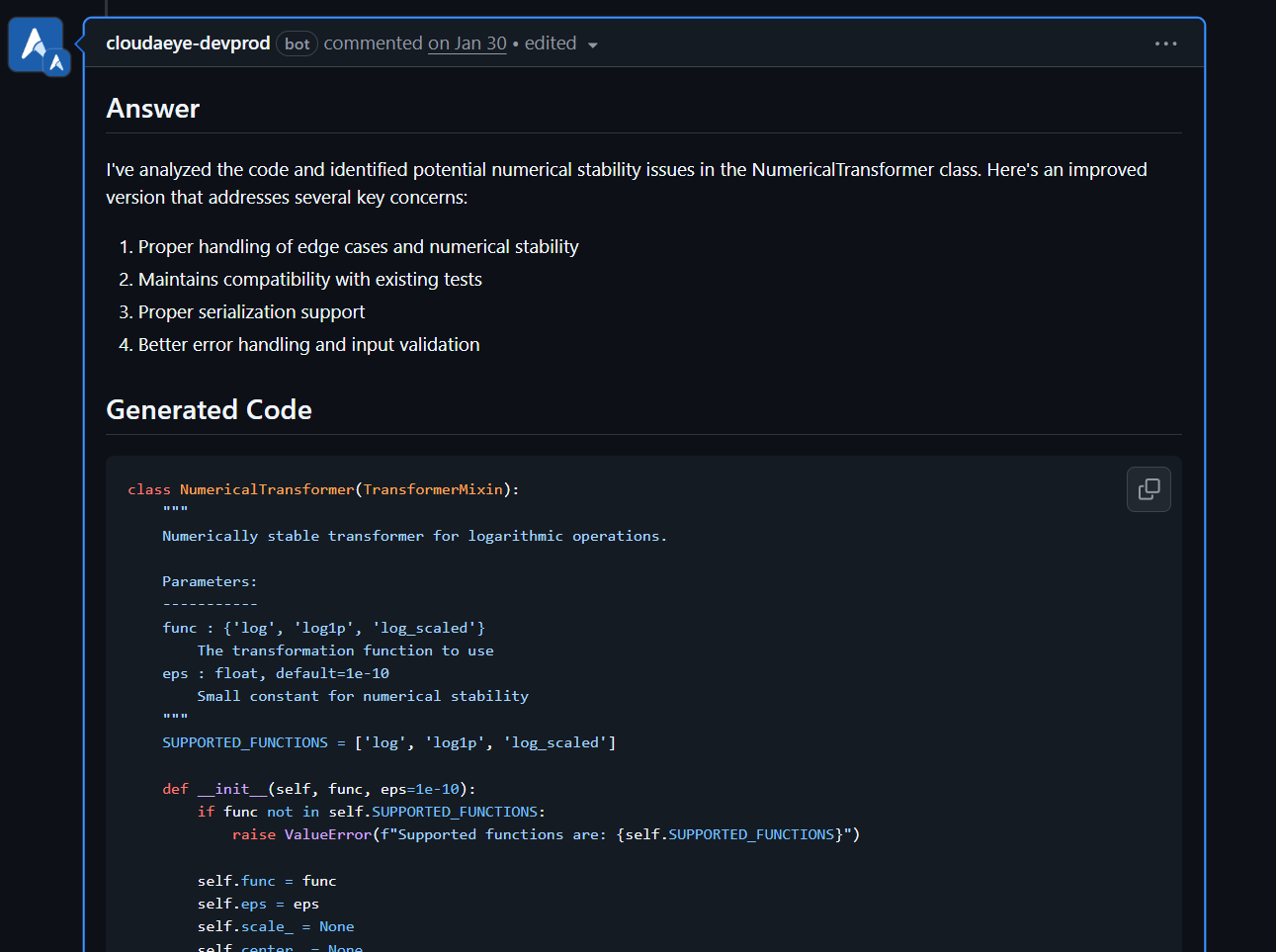
Automatically receive intelligent code fixes to streamline resolution and reduce cognitive load. Let the AI agent generate the required code changes, complete with context from your existing codebase. Use seamlessly in your IDE or right from GitHub.
Auto-generate comprehensive docstrings and comments to improve code maintainability and simplify onboarding for new developers. Use it without leaving your IDE or GitHub.
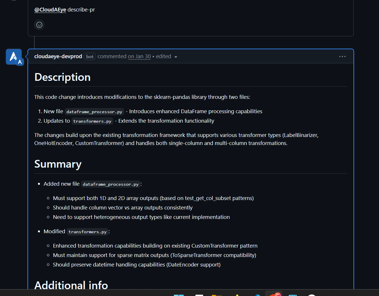
Auto-generate a detailed PR description for code changes in the current PR. Integrated directly with GitHub workflows — no context switching required.
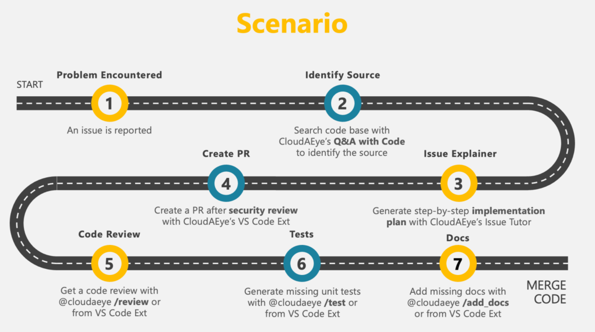
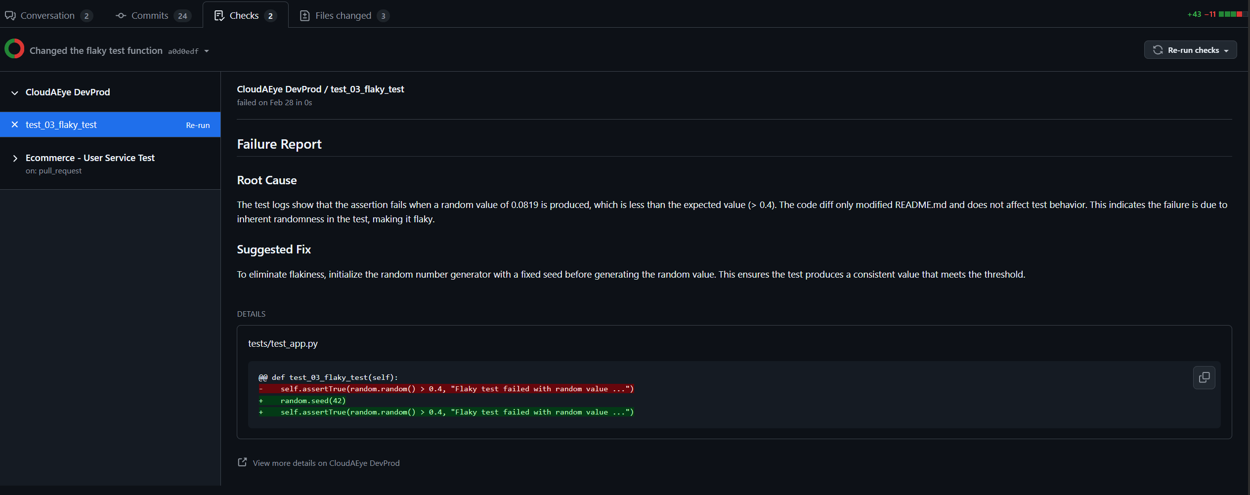
Stop wasting hours debugging CI/CD failures. Our AI-powered engine delivers instant root cause analysis (RCA) for every test failure — right in your GitHub pull request, as a comment. It also automatically handles flaky tests (those annoying failures that happen without code changes) and streamlines test triaging by grouping and categorizing failures for faster resolution.
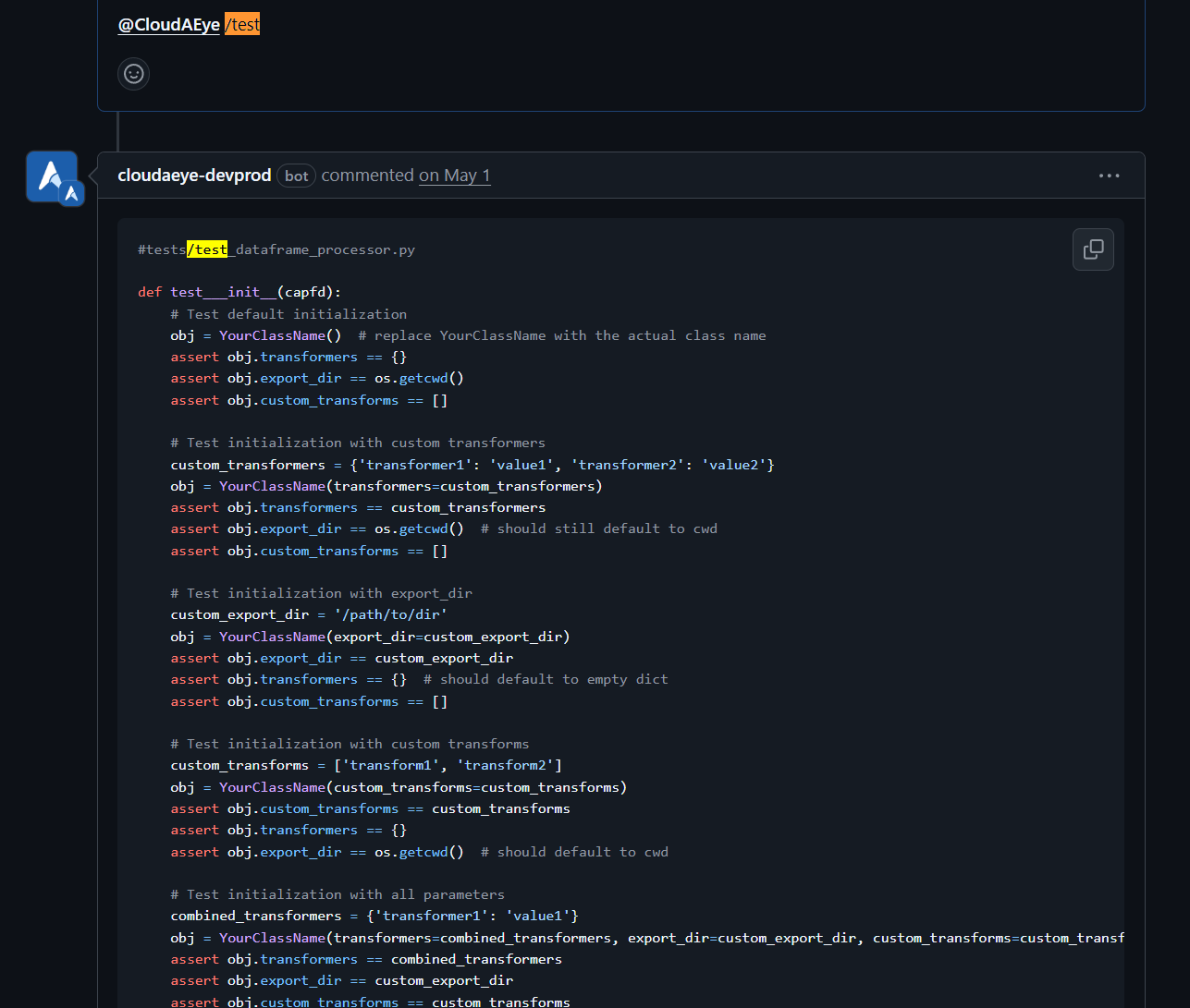
Automatically generate and update unit tests with every code change. CloudAEye covers edge and negative cases to help you achieve 100% test coverage effortlessly. Use seamlessly in your IDE or right from GitHub.
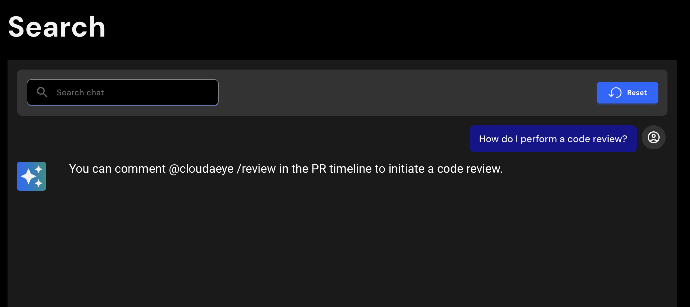
Debug and understand large enterprise codebases spanning hundreds of repositories. Ask "where" and "why" questions in natural language to pinpoint problems quickly in GitHub or the chatbot interface.
Get step-by-step implementation guidance for any Jira or GitHub issue. The AI provides a technical breakdown and code suggestions.
Make all internal and external documentation (Confluence, Docs, PDFs, Slack, YouTube) searchable. Digitize tribal knowledge and find answers instantly.
CloudAEye provides enterprise-grade security, broad integration support, and cutting-edge AI to deliver reliable, secure, and intelligent development tools.
Code is reviewed against OWASP top 10 vulnerability detection and the Agentic Security Initiative (ASI) by default. Build secure applications from the first line of code.
Native support for your stack. We understand CNCF projects, top open-source libraries, and 3rd party APIs to provide truly accurate analysis.
Our autonomous agents don't just find problems—they reason, plan, and execute solutions. This is more than automation; it's a true developer companion.
Stay updated with the latest insights, tutorials, and industry trends in AI-powered development.

Join us at industry events and catch up on our previous talks and webinars.
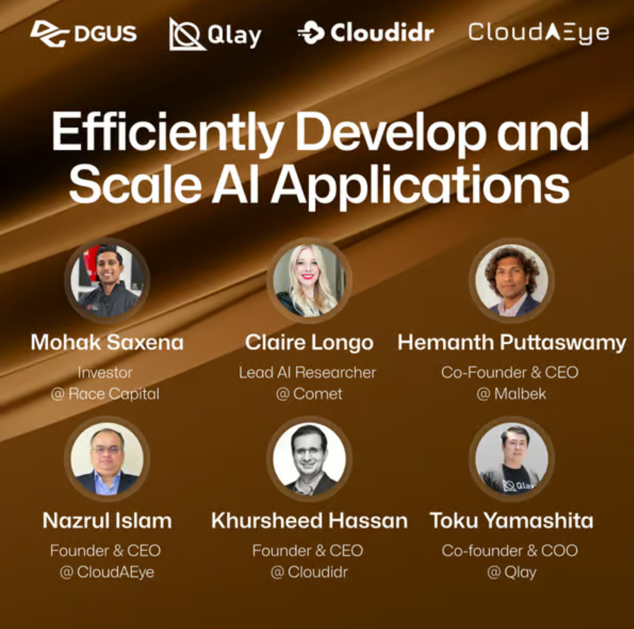
Join industry leaders for an interactive panel discussion on the practical challenges and solutions for building production-ready AI applications at scale. Learn from companies solving real infrastructure, development, and talent challenges in the AI space.
CloudAEye showcased AI-powered developer tools at the premier AI development conference as a top 20 startups, demonstrating how AI agents can revolutionize software development workflows.

CloudAEye was part of the vibrant tech gathering at Collision Conf in Toronto! The event achieved remarkable scale, attracting more than 37,000 participants and 1,600 companies, highlighted by a series of impactful keynote presentations.
Experience the power of AI-driven development tools. Join other developers who are already shipping code 4x faster with CloudAEye's intelligent agents.